CARTOframes

A Python package for integrating CARTO maps, analysis, and data services into data science workflows.

Python data analysis workflows often rely on the de facto standards pandas and Jupyter notebooks. Integrating CARTO into this workflow saves data scientists time and energy by not having to export datasets as files or retain multiple copies of the data. Instead, CARTOframes give the ability to communicate reproducible analysis while providing the ability to gain from CARTO’s services like hosted, dynamic or static maps and Data Observatory augmentation.

Features

• Write pandas DataFrames to CARTO tables
• Read CARTO tables and queries into pandas DataFrames
• Create customizable, interactive CARTO maps in a Jupyter notebook
• Interact with CARTO’s Data Observatory
• Use CARTO’s spatially-enabled database for analysis
• Try it out without needing a CARTO account by using the Examples functionality

Common Uses

• Visualize spatial data programmatically as matplotlib images or embedded interactive maps
• Perform cloud-based spatial data processing using CARTO’s analysis tools
• Extract, transform, and Load (ETL) data using the Python ecosystem for getting data into and out of CARTO
• Data Services integrations using CARTO’s Data Observatory and other Data Services APIs

Try it out

The easiest way to try out cartoframes is to use the cartoframes example notebooks running in binder: https://mybinder.org/v2/gh/CartoDB/cartoframes/master?filepath=examples If you already have an API key, you can follow along and complete all of the example notebooks.

If you do not have an API key, you can use the Example Context to read the example data, make maps, and run arbitrary queries from the datasets there. The best place to get started is in the “Example Datasets” notebook found when running binder or downloading from the examples directory in the cartoframes GitHub repository.

Note

The example context only provides read access, so not all cartoframes features are available. For full access, Start a free 30 day trial or get free access with a GitHub Student Developer Pack.

More info

• Complete documentation: http://cartoframes.readthedocs.io/en/latest/
• Source code: https://github.com/CartoDB/cartoframes
• bug tracker / feature requests: https://github.com/CartoDB/cartoframes/issues

Note

cartoframes users must have a CARTO API key for most cartoframes functionality. For example, writing DataFrames to an account, reading from private tables, and visualizing data on maps all require an API key. CARTO provides API keys for education and nonprofit uses, among others. Request access at support@carto.com. API key access is also given through GitHub’s Student Developer Pack.

Install Instructions

To install cartoframes on your machine, do the following to install the latest version:

$ pip install cartoframes

cartoframes is continuously tested on Python versions 2.7, 3.5, and 3.6. It is recommended to use cartoframes in Jupyter Notebooks (pip install jupyter). See the example usage section below or notebooks in the examples directory for using cartoframes in that environment.

Virtual Environment

Using virtualenv

Make sure your virtualenv package is installed and up-to-date. See the official Python packaging page for more information.

To setup cartoframes and Jupyter in a virtual environment:

$ virtualenv venv
$ source venv/bin/activate
(venv) $ pip install cartoframes jupyter
(venv) $ jupyter notebook

Then create a new notebook and try the example code snippets below with tables that are in your CARTO account.

Using pipenv

Alternatively, pipenv provides an easy way to manage virtual environments. The steps below are:

1. Create a virtual environment with Python 3.4+ (recommended instead of Python 2.7)
2. Install cartoframes and Jupyter (optional) into the virtual environment
3. Enter the virtual environment
4. Launch a Jupyter notebook server

$ pipenv --three
$ pipenv install cartoframes jupyter
$ pipenv shell

Next, run a Python kernel by typing $ python, $ jupyter notebook, or however you typically run Python.

Native pip

If you install packages at a system level, you can install cartoframes with:

$ pip install cartoframes

Example usage

Data workflow

Get table from CARTO, make changes in pandas, sync updates with CARTO:

import cartoframes
# `base_url`s are of the form `https://{username}.carto.com/` for most users
cc = cartoframes.CartoContext(base_url='https://eschbacher.carto.com/',
                              api_key=APIKEY)

# read a table from your CARTO account to a DataFrame
df = cc.read('brooklyn_poverty_census_tracts')

# do fancy pandas operations (add/drop columns, change values, etc.)
df['poverty_per_pop'] = df['poverty_count'] / df['total_population']

# updates CARTO table with all changes from this session
cc.write(df, 'brooklyn_poverty_census_tracts', overwrite=True)

Write an existing pandas DataFrame to CARTO.

import pandas as pd
import cartoframes
df = pd.read_csv('acadia_biodiversity.csv')
cc = cartoframes.CartoContext(base_url=BASEURL,
                              api_key=APIKEY)
cc.write(df, 'acadia_biodiversity')

Map workflow

The following will embed a CARTO map in a Jupyter notebook, allowing for custom styling of the maps driven by TurboCARTO and CARTOColors. See the CARTOColors wiki for a full list of available color schemes.

from cartoframes import Layer, BaseMap, styling
cc = cartoframes.CartoContext(base_url=BASEURL,
                              api_key=APIKEY)
cc.map(layers=[BaseMap('light'),
               Layer('acadia_biodiversity',
                     color={'column': 'simpson_index',
                            'scheme': styling.tealRose(5)}),
               Layer('peregrine_falcon_nest_sites',
                     size='num_eggs',
                     color={'column': 'bird_id',
                            'scheme': styling.vivid(10)})],
       interactive=True)

Note

Legends are under active development. See https://github.com/CartoDB/cartoframes/pull/184 for more information. To try out that code, install cartoframes as:

pip install git+https://github.com/cartodb/cartoframes.git@add-legends-v1#egg=cartoframes

Data Observatory

Interact with CARTO’s Data Observatory:

import cartoframes
cc = cartoframes.CartoContext(BASEURL, APIKEY)

# total pop, high school diploma (normalized), median income, poverty status (normalized)
# See Data Observatory catalog for codes: https://cartodb.github.io/bigmetadata/index.html
data_obs_measures = [{'numer_id': 'us.census.acs.B01003001'},
                     {'numer_id': 'us.census.acs.B15003017',
                      'normalization': 'predenominated'},
                     {'numer_id': 'us.census.acs.B19013001'},
                     {'numer_id': 'us.census.acs.B17001002',
                      'normalization': 'predenominated'},]
df = cc.data('transactions', data_obs_measures)

CARTO Credential Management

Typical usage

The most common way to input credentials into cartoframes is through the CartoContext, as below. Replace {your_user_name} with your CARTO username and {your_api_key} with your API key, which you can find at https://{your_user_name}.carto.com/your_apps.

from cartoframes import CartoContext
cc = CartoContext(
    base_url='https://{your_user_name}.carto.com',
    api_key='{your_api_key}'
)

You can also set your credentials using the Credentials class:

from cartoframes import Credentials, CartoContext
cc = CartoContext(
    creds=Credentials(key='{your_api_key}', username='{your_user_name}')
)

Save/update credentials for later use

from cartoframes import Credentials, CartoContext
creds = Credentials(username='eschbacher', key='abcdefg')
creds.save()  # save credentials for later use (not dependent on Python session)

Once you save your credentials, you can get started in future sessions more quickly:

from cartoframes import CartoContext
cc = CartoContext()  # automatically loads credentials if previously saved

Experimental features

CARTOframes includes experimental features that we are testing for future releases into cartoframes core. These features exist as separate modules in contrib. These features are stand-alone other than sometimes relying on some cartoframes utilities, etc. Contrib features will also change often and without notice, so they should never be used in a production environment.

To import an experimental feature, like vector maps, do the following:

from cartoframes.contrib import vector
from cartoframes import CartoContext

cc = CartoContext()
vector.vmap([vector.Layer('<table name>'), ], context=cc)

CARTOframes Functionality

CartoContext

class cartoframes.context.CartoContext(base_url=None, api_key=None, creds=None, session=None, verbose=0)

CartoContext class for authentication with CARTO and high-level operations such as reading tables from CARTO into dataframes, writing dataframes to CARTO tables, creating custom maps from dataframes and CARTO tables, and augmenting data using CARTO’s Data Observatory. Future methods will interact with CARTO’s services like routing, geocoding, and isolines, PostGIS backend for spatial processing, and much more.

Manages connections with CARTO for data and map operations. Modeled after SparkContext.

There are two ways of authenticating against a CARTO account:

1. Setting the base_url and api_key directly in CartoContext. This method is easier.:

   cc = CartoContext(
       base_url='https://eschbacher.carto.com',
       api_key='abcdefg')
   

2. By passing a Credentials instance in CartoContext’s creds keyword argument. This method is more flexible.:

   from cartoframes import Credentials
   creds = Credentials(user='eschbacher', key='abcdefg')
   cc = CartoContext(creds=creds)
   

creds

Credentials instance

Type:Credentials

Parameters:

• base_url (str) – Base URL of CARTO user account. Cloud-based accounts should use the form https://{username}.carto.com (e.g., https://eschbacher.carto.com for user eschbacher) whether on a personal or multi-user account. On-premises installation users should ask their admin.
• api_key (str) – CARTO API key.
• creds (Credentials) – A Credentials instance can be used in place of a base_url/api_key combination.
• session (requests.Session, optional) – requests session. See requests documentation for more information.
• verbose (bool, optional) – Output underlying process states (True), or suppress (False, default)

Returns:

A CartoContext object that is authenticated against the user’s CARTO account.

Return type:

CartoContext

Example

Create a CartoContext object for a cloud-based CARTO account.

import cartoframes
# if on prem, format is '{host}/user/{username}'
BASEURL = 'https://{}.carto.com/'.format('your carto username')
APIKEY = 'your carto api key'
cc = cartoframes.CartoContext(BASEURL, APIKEY)

Tip

If using cartoframes with an on premises CARTO installation, sometimes it is necessary to disable SSL verification depending on your system configuration. You can do this using a requests Session object as follows:

import cartoframes
from requests import Session
session = Session()
session.verify = False

# on prem host (e.g., an IP address)
onprem_host = 'your on prem carto host'

cc = cartoframes.CartoContext(
    base_url='{host}/user/{user}'.format(
        host=onprem_host,
        user='your carto username'),
    api_key='your carto api key',
    session=session
)

write(df, table_name, temp_dir=SYSTEM_TMP_PATH, overwrite=False, lnglat=None, encode_geom=False, geom_col=None, **kwargs)

Write a DataFrame to a CARTO table.

Examples

Write a pandas DataFrame to CARTO.

cc.write(df, 'brooklyn_poverty', overwrite=True)

Scrape an HTML table from Wikipedia and send to CARTO with content guessing to create a geometry from the country column. This uses a CARTO Import API param content_guessing parameter.

url = 'https://en.wikipedia.org/wiki/List_of_countries_by_life_expectancy'
# retrieve first HTML table from that page
df = pd.read_html(url, header=0)[0]
# send to carto, let it guess polygons based on the 'country'
#   column. Also set privacy to 'public'
cc.write(df, 'life_expectancy',
         content_guessing=True,
         privacy='public')
cc.map(layers=Layer('life_expectancy',
                    color='both_sexes_life_expectancy'))

Parameters:

• df (pandas.DataFrame) – DataFrame to write to table_name in user CARTO account
• table_name (str) – Table to write df to in CARTO.
• temp_dir (str, optional) – Directory for temporary storage of data that is sent to CARTO. Defaults are defined by appdirs.
• overwrite (bool, optional) – Behavior for overwriting table_name if it exits on CARTO. Defaults to False.
• lnglat (tuple, optional) – lng/lat pair that can be used for creating a geometry on CARTO. Defaults to None. In some cases, geometry will be created without specifying this. See CARTO’s Import API for more information.
• encode_geom (bool, optional) – Whether to write geom_col to CARTO as the_geom.
• geom_col (str, optional) – The name of the column where geometry information is stored. Used in conjunction with encode_geom.
• **kwargs –

  Keyword arguments to control write operations. Options are:

  • compression to set compression for files sent to CARTO. This will cause write speedups depending on the dataset. Options are None (no compression, default) or gzip.
  • Some arguments from CARTO’s Import API. See the params listed in the documentation for more information. For example, when using content_guessing=’true’, a column named ‘countries’ with country names will be used to generate polygons for each country. Another use is setting the privacy of a dataset. To avoid unintended consequences, avoid file, url, and other similar arguments.

Returns:

BatchJobStatus or None: If lnglat flag is set and the DataFrame has more than 100,000 rows, a BatchJobStatus instance is returned. Otherwise, None.

Note

DataFrame indexes are changed to ordinary columns. CARTO creates an index called cartodb_id for every table that runs from 1 to the length of the DataFrame.

tables()

List all tables in user’s CARTO account

Returns:list of Table

read(table_name, limit=None, index='cartodb_id', decode_geom=False, shared_user=None)

Read a table from CARTO into a pandas DataFrames.

Parameters:

• table_name (str) – Name of table in user’s CARTO account.
• limit (int, optional) – Read only limit lines from table_name. Defaults to None, which reads the full table.
• index (str, optional) – Not currently in use.
• decode_geom (bool, optional) – Decodes CARTO’s geometries into a Shapely object that can be used, for example, in GeoPandas.
• shared_user (str, optional) – If a table has been shared with you, specify the user name (schema) who shared it.

Returns:

DataFrame representation of table_name from CARTO.

Return type:

pandas.DataFrame

Example

import cartoframes
cc = cartoframes.CartoContext(BASEURL, APIKEY)
df = cc.read('acadia_biodiversity')

delete(table_name)

Delete a table in user’s CARTO account.

Parameters:table_name (str) – Name of table to delete Returns:None

query(query, table_name=None, decode_geom=False)

Pull the result from an arbitrary SQL query from a CARTO account into a pandas DataFrame. Can also be used to perform database operations (creating/dropping tables, adding columns, updates, etc.).

Parameters:

• query (str) – Query to run against CARTO user database. This data will then be converted into a pandas DataFrame.
• table_name (str, optional) – If set, this will create a new table in the user’s CARTO account that is the result of the query. Defaults to None (no table created).
• decode_geom (bool, optional) – Decodes CARTO’s geometries into a Shapely object that can be used, for example, in GeoPandas.

Returns:

DataFrame representation of query supplied. Pandas data types are inferred from PostgreSQL data types. In the case of PostgreSQL date types, dates are attempted to be converted, but on failure a data type ‘object’ is used.

Return type:

pandas.DataFrame

Examples

Query a table in CARTO and write a new table that is result of query. This query gets the 10 highest values from a table and returns a dataframe, as well as creating a new table called ‘top_ten’ in the CARTO account.

topten_df = cc.query(
    '''
      SELECT * FROM
      my_table
      ORDER BY value_column DESC
      LIMIT 10
    ''',
    table_name='top_ten'
)

This query joins points to polygons based on intersection, and aggregates by summing the values of the points in each polygon. The query returns a dataframe, with a geometry column that contains polygons and also creates a new table called ‘points_aggregated_to_polygons’ in the CARTO account.

points_aggregated_to_polygons = cc.query(
    '''
      SELECT polygons.*, sum(points.values)
      FROM polygons JOIN points
      ON ST_Intersects(points.the_geom, polygons.the_geom)
      GROUP BY polygons.the_geom, polygons.cartodb_id
    ''',
    table_name='points_aggregated_to_polygons',
    decode_geom=True
)

map(**kwargs)

Produce a CARTO map visualizing data layers.

Examples

Create a map with two data Layers, and one BaseMap layer:

import cartoframes
from cartoframes import Layer, BaseMap, styling
cc = cartoframes.CartoContext(BASEURL, APIKEY)
cc.map(layers=[BaseMap(),
               Layer('acadia_biodiversity',
                     color={'column': 'simpson_index',
                            'scheme': styling.tealRose(7)}),
               Layer('peregrine_falcon_nest_sites',
                     size='num_eggs',
                     color={'column': 'bird_id',
                            'scheme': styling.vivid(10))],
       interactive=True)

Create a snapshot of a map at a specific zoom and center:

cc.map(layers=Layer('acadia_biodiversity',
                    color='simpson_index'),
       interactive=False,
       zoom=14,
       lng=-68.3823549,
       lat=44.3036906)

Parameters:

• layers (list, optional) –

  List of zero or more of the following:

  • Layer: cartoframes Layer object for visualizing data from a CARTO table. See Layer for all styling options.
  • BaseMap: Basemap for contextualizng data layers. See BaseMap for all styling options.
  • QueryLayer: Layer from an arbitrary query. See QueryLayer for all styling options.
• interactive (bool, optional) – Defaults to True to show an interactive slippy map. Setting to False creates a static map.
• zoom (int, optional) – Zoom level of map. Acceptable values are usually in the range 0 to 19. 0 has the entire earth on a single tile (256px square). Zoom 19 is the size of a city block. Must be used in conjunction with lng and lat. Defaults to a view to have all data layers in view.
• lat (float, optional) – Latitude value for the center of the map. Must be used in conjunction with zoom and lng. Defaults to a view to have all data layers in view.
• lng (float, optional) – Longitude value for the center of the map. Must be used in conjunction with zoom and lat. Defaults to a view to have all data layers in view.
• size (tuple, optional) – List of pixel dimensions for the map. Format is (width, height). Defaults to (800, 400).
• ax – matplotlib axis on which to draw the image. Only used when interactive is False.

Returns:

Interactive maps are rendered as HTML in an iframe, while static maps are returned as matplotlib Axes objects or IPython Image.

Return type:

IPython.display.HTML or matplotlib Axes

data_boundaries(boundary=None, region=None, decode_geom=False, timespan=None, include_nonclipped=False)

Find all boundaries available for the world or a region. If boundary is specified, get all available boundary polygons for the region specified (if any). This method is espeically useful for getting boundaries for a region and, with CartoContext.data and CartoContext.data_discovery, getting tables of geometries and the corresponding raw measures. For example, if you want to analyze how median income has changed in a region (see examples section for more).

Examples

Find all boundaries available for Australia. The columns geom_name gives us the name of the boundary and geom_id is what we need for the boundary argument.

import cartoframes
cc = cartoframes.CartoContext('base url', 'api key')
au_boundaries = cc.data_boundaries(region='Australia')
au_boundaries[['geom_name', 'geom_id']]

Get the boundaries for Australian Postal Areas and map them.

from cartoframes import Layer
au_postal_areas = cc.data_boundaries(boundary='au.geo.POA')
cc.write(au_postal_areas, 'au_postal_areas')
cc.map(Layer('au_postal_areas'))

Get census tracts around Idaho Falls, Idaho, USA, and add median income from the US census. Without limiting the metadata, we get median income measures for each census in the Data Observatory.

cc = cartoframes.CartoContext('base url', 'api key')
# will return DataFrame with columns `the_geom` and `geom_ref`
tracts = cc.data_boundaries(
    boundary='us.census.tiger.census_tract',
    region=[-112.096642,43.429932,-111.974213,43.553539])
# write geometries to a CARTO table
cc.write(tracts, 'idaho_falls_tracts')
# gather metadata needed to look up median income
median_income_meta = cc.data_discovery(
    'idaho_falls_tracts',
    keywords='median income',
    boundaries='us.census.tiger.census_tract')
# get median income data and original table as new dataframe
idaho_falls_income = cc.data(
    'idaho_falls_tracts',
    median_income_meta,
    how='geom_refs')
# overwrite existing table with newly-enriched dataframe
cc.write(idaho_falls_income,
         'idaho_falls_tracts',
         overwrite=True)

Parameters:

• boundary (str, optional) – Boundary identifier for the boundaries that are of interest. For example, US census tracts have a boundary ID of us.census.tiger.census_tract, and Brazilian Municipios have an ID of br.geo.municipios. Find IDs by running CartoContext.data_boundaries without any arguments, or by looking in the Data Observatory catalog.
• region (str, optional) –

  Region where boundary information or, if boundary is specified, boundary polygons are of interest. region can be one of the following:

  • table name (str): Name of a table in user’s CARTO account
  • bounding box (list of float): List of four values (two lng/lat pairs) in the following order: western longitude, southern latitude, eastern longitude, and northern latitude. For example, Switzerland fits in [5.9559111595,45.8179931641,10.4920501709,47.808380127]

• timespan (str, optional) – Specific timespan to get geometries from. Defaults to use the most recent. See the Data Observatory catalog for more information.
• decode_geom (bool, optional) – Whether to return the geometries as Shapely objects or keep them encoded as EWKB strings. Defaults to False.
• include_nonclipped (bool, optional) – Optionally include non-shoreline-clipped boundaries. These boundaries are the raw boundaries provided by, for example, US Census Tiger.

Returns:

If boundary is specified, then all available boundaries and accompanying geom_refs in region (or the world if region is None or not specified) are returned. If boundary is not specified, then a DataFrame of all available boundaries in region (or the world if region is None)

Return type:

pandas.DataFrame

data_discovery(region, keywords=None, regex=None, time=None, boundaries=None, include_quantiles=False)

Discover Data Observatory measures. This method returns the full Data Observatory metadata model for each measure or measures that match the conditions from the inputs. The full metadata in each row uniquely defines a measure based on the timespan, geographic resolution, and normalization (if any). Read more about the metadata response in Data Observatory documentation.

Internally, this method finds all measures in region that match the conditions set in keywords, regex, time, and boundaries (if any of them are specified). Then, if boundaries is not specified, a geographical resolution for that measure will be chosen subject to the type of region specified:

1. If region is a table name, then a geographical resolution that is roughly equal to region size / number of subunits.
2. If region is a country name or bounding box, then a geographical resolution will be chosen roughly equal to region size / 500.

Since different measures are in some geographic resolutions and not others, different geographical resolutions for different measures are oftentimes returned.

Tip

To remove the guesswork in how geographical resolutions are selected, specify one or more boundaries in boundaries. See the boundaries section for each region in the Data Observatory catalog.

The metadata returned from this method can then be used to create raw tables or for augmenting an existing table from these measures using CartoContext.data. For the full Data Observatory catalog, visit https://cartodb.github.io/bigmetadata/. When working with the metadata DataFrame returned from this method, be careful to only remove rows not columns as CartoContext.data <cartoframes.context.CartoContext.data> generally needs the full metadata.

Note

Narrowing down a discovery query using the keywords, regex, and time filters is important for getting a manageable metadata set. Besides there being a large number of measures in the DO, a metadata response has acceptable combinations of measures with demonimators (normalization and density), and the same measure from other years.

For example, setting the region to be United States counties with no filter values set will result in many thousands of measures.

Examples

Get all European Union measures that mention freight.

meta = cc.data_discovery('European Union',
                         keywords='freight',
                         time='2010')
print(meta['numer_name'].values)

Parameters:

• region (str or list of float) –

  Information about the region of interest. region can be one of three types:

  • region name (str): Name of region of interest. Acceptable values are limited to: ‘Australia’, ‘Brazil’, ‘Canada’, ‘European Union’, ‘France’, ‘Mexico’, ‘Spain’, ‘United Kingdom’, ‘United States’.
  • table name (str): Name of a table in user’s CARTO account with geometries. The region will be the bounding box of the table.

    Note

    If a table name is also a valid Data Observatory region name, the Data Observatory name will be chosen over the table.

  • bounding box (list of float): List of four values (two lng/lat pairs) in the following order: western longitude, southern latitude, eastern longitude, and northern latitude. For example, Switzerland fits in [5.9559111595,45.8179931641,10.4920501709,47.808380127]

  Note

  Geometry levels are generally chosen by subdividing the region into the next smallest administrative unit. To override this behavior, specify the boundaries flag. For example, set boundaries to 'us.census.tiger.census_tract' to choose US census tracts.

• keywords (str or list of str, optional) – Keyword or list of keywords in measure description or name. Response will be matched on all keywords listed (boolean or).
• regex (str, optional) – A regular expression to search the measure descriptions and names. Note that this relies on PostgreSQL’s case insensitive operator ~*. See PostgreSQL docs for more information.
• boundaries (str or list of str, optional) – Boundary or list of boundaries that specify the measure resolution. See the boundaries section for each region in the Data Observatory catalog.
• include_quantiles (bool, optional) – Include quantiles calculations which are a calculation of how a measure compares to all measures in the full dataset. Defaults to False. If True, quantiles columns will be returned for each column which has it pre-calculated.

Returns:

A dataframe of the complete metadata model for specific measures based on the search parameters.

Return type:

pandas.DataFrame

Raises:

• ValueError – If region is a list and does not consist of four elements, or if region is not an acceptable region
• CartoException – If region is not a table in user account

data(table_name, metadata, persist_as=None, how='the_geom')

Get an augmented CARTO dataset with Data Observatory measures. Use CartoContext.data_discovery to search for available measures, or see the full Data Observatory catalog. Optionally persist the data as a new table.

Example

Get a DataFrame with Data Observatory measures based on the geometries in a CARTO table.

cc = cartoframes.CartoContext(BASEURL, APIKEY)
median_income = cc.data_discovery('transaction_events',
                                  regex='.*median income.*',
                                  time='2011 - 2015')
df = cc.data('transaction_events',
             median_income)

Pass in cherry-picked measures from the Data Observatory catalog. The rest of the metadata will be filled in, but it’s important to specify the geographic level as this will not show up in the column name.

median_income = [{'numer_id': 'us.census.acs.B19013001',
                  'geom_id': 'us.census.tiger.block_group',
                  'numer_timespan': '2011 - 2015'}]
df = cc.data('transaction_events', median_income)

Parameters:

• table_name (str) – Name of table on CARTO account that Data Observatory measures are to be added to.
• metadata (pandas.DataFrame) – List of all measures to add to table_name. See CartoContext.data_discovery outputs for a full list of metadata columns.
• persist_as (str, optional) – Output the results of augmenting table_name to persist_as as a persistent table on CARTO. Defaults to None, which will not create a table.
• how (str, optional) – Not fully implemented. Column name for identifying the geometry from which to fetch the data. Defaults to the_geom, which results in measures that are spatially interpolated (e.g., a neighborhood boundary’s population will be calculated from underlying census tracts). Specifying a column that has the geometry identifier (for example, GEOID for US Census boundaries), results in measures directly from the Census for that GEOID but normalized how it is specified in the metadata.

Returns:

A DataFrame representation of table_name which has new columns for each measure in metadata.

Return type:

pandas.DataFrame

Raises:

• NameError – If the columns in table_name are in the suggested_name column of metadata.
• ValueError – If metadata object is invalid or empty, or if the number of requested measures exceeds 50.
• CartoException – If user account consumes all of Data Observatory quota

Map Layer Classes

class cartoframes.layer.BaseMap(source='voyager', labels='back', only_labels=False)

Layer object for adding basemaps to a cartoframes map.

Example

Add a custom basemap to a cartoframes map.

import cartoframes
from cartoframes import BaseMap, Layer
cc = cartoframes.CartoContext(BASEURL, APIKEY)
cc.map(layers=[BaseMap(source='light', labels='front'),
               Layer('acadia_biodiversity')])

Parameters:

• source (str, optional) – One of light or dark. Defaults to voyager. Basemaps come from https://carto.com/location-data-services/basemaps/
• labels (str, optional) – One of back, front, or None. Labels on the front will be above the data layers. Labels on back will be underneath the data layers but on top of the basemap. Setting labels to None will only show the basemap.
• only_labels (bool, optional) – Whether to show labels or not.

class cartoframes.layer.Layer(table_name, source=None, overwrite=False, time=None, color=None, size=None, opacity=None, tooltip=None, legend=None)

A cartoframes Data Layer based on a specific table in user’s CARTO database. This layer class is used for visualizing individual datasets with CartoContext.map’s layers keyword argument.

Example

import cartoframes
from cartoframes import QueryLayer, styling
cc = cartoframes.CartoContext(BASEURL, APIKEY)
cc.map(layers=[Layer('fantastic_sql_table',
                     size=7,
                     color={'column': 'mr_fox_sightings',
                            'scheme': styling.prism(10)})])

Parameters:

• table_name (str) – Name of table in CARTO account
• Styling – See QueryLayer
• a full list of all arguments arguments for styling this map data (for) –
• layer. –
• source (pandas.DataFrame, optional) – Not currently implemented
• overwrite (bool, optional) – Not currently implemented

class cartoframes.layer.QueryLayer(query, time=None, color=None, size=None, opacity=None, tooltip=None, legend=None)

cartoframes data layer based on an arbitrary query to the user’s CARTO database. This layer class is useful for offloading processing to the cloud to do some of the following:

• Visualizing spatial operations using PostGIS and PostgreSQL, which is the database underlying CARTO
• Performing arbitrary relational database queries (e.g., complex JOINs in SQL instead of in pandas)
• Visualizing a subset of the data (e.g., SELECT * FROM table LIMIT 1000)

Used in the layers keyword in CartoContext.map.

Example

Underlay a QueryLayer with a complex query below a layer from a table. The QueryLayer is colored by the calculated column abs_diff, and points are sized by the column i_measure.

import cartoframes
from cartoframes import QueryLayer, styling
cc = cartoframes.CartoContext(BASEURL, APIKEY)
cc.map(layers=[QueryLayer('''
                          WITH i_cte As (
                            SELECT
                                ST_Buffer(the_geom::geography, 500)::geometry As the_geom,
                                cartodb_id,
                                measure,
                                date
                              FROM interesting_data
                             WHERE date > '2017-04-19'
                          )
                          SELECT
                             i.cartodb_id, i.the_geom,
                             ST_Transform(i.the_geom, 3857) AS the_geom_webmercator,
                             abs(i.measure - j.measure) AS abs_diff,
                             i.measure AS i_measure
                            FROM i_cte AS i
                            JOIN awesome_data AS j
                              ON i.event_id = j.event_id
                           WHERE j.measure IS NOT NULL
                             AND j.date < '2017-04-29'
                          ''',
                          color={'column': 'abs_diff',
                                 'scheme': styling.sunsetDark(7)},
                          size='i_measure'),
               Layer('fantastic_sql_table')])

Parameters:

• query (str) – Query to expose data on a map layer. At a minimum, a query needs to have the columns cartodb_id, the_geom, and the_geom_webmercator for the map to display. Read more about queries in CARTO’s docs.
• time (dict or str, optional) –

  Time-based style to apply to layer.

  If time is a str, it must be the name of a column which has a data type of datetime or float.

  from cartoframes import QueryLayer
  l = QueryLayer('SELECT * FROM acadia_biodiversity',
                 time='bird_sighting_time')
  

  If time is a dict, the following keys are options:

  • column (str, required): Column for animating map, which must be of type datetime or float.
  • method (str, optional): Type of aggregation method for operating on Torque TileCubes. Must be one of avg, sum, or another PostgreSQL aggregate functions with a numeric output. Defaults to count.
  • cumulative (bool, optional): Whether to accumulate points over time (True) or not (False, default)
  • frames (int, optional): Number of frames in the animation. Defaults to 256.
  • duration (int, optional): Number of seconds in the animation. Defaults to 30.
  • trails (int, optional): Number of trails after the incidence of a point. Defaults to 2.

  from cartoframes import Layer
  l = Layer('acadia_biodiversity',
            time={
                'column': 'bird_sighting_time',
                'cumulative': True,
                'frames': 128,
                'duration': 15
            })
  

• color (dict or str, optional) –

  Color style to apply to map. For example, this can be used to change the color of all geometries in this layer, or to create a graduated color or choropleth map.

  If color is a str, there are two options:

  • A column name to style by to create, for example, a choropleth map if working with polygons. The default classification is quantiles for quantitative data and category for qualitative data.
  • A hex value or web color name.

  # color all geometries red (#F00)
  from cartoframes import Layer
  l = Layer('acadia_biodiversity',
            color='red')
  
  # color on 'num_eggs' (using defalt color scheme and quantification)
  l = Layer('acadia_biodiversity',
            color='num_eggs')
  

  If color is a dict, the following keys are options, with values described:

  • column (str): Column used for the basis of styling
  • scheme (dict, optional): Scheme such as styling.sunset(7) from the styling module of cartoframes that exposes CARTOColors. Defaults to mint scheme for quantitative data and bold for qualitative data. More control is given by using styling.scheme.

    If you wish to define a custom scheme outside of CARTOColors, it is recommended to use the styling.custom utility function.

  from cartoframes import QueryLayer, styling
  l = QueryLayer('SELECT * FROM acadia_biodiversity',
                 color={
                     'column': 'simpson_index',
                     'scheme': styling.mint(7, bin_method='equal')
                 })
  

• size (dict or int, optional) –

  Size style to apply to point data.

  If size is an int, all points are sized by this value.

  from cartoframes import QueryLayer
  l = QueryLayer('SELECT * FROM acadia_biodiversity',
                 size=7)
  

  If size is a str, this value is interpreted as a column, and the points are sized by the value in this column. The classification method defaults to quantiles, with a min size of 5, and a max size of 5. Use the dict input to override these values.

  from cartoframes import Layer
  l = Layer('acadia_biodiversity',
            size='num_eggs')
  

  If size is a dict, the follow keys are options, with values described as:

  • column (str): Column to base sizing of points on
  • bin_method (str, optional): Quantification method for dividing data range into bins. Must be one of the methods in BinMethod (excluding category).
  • bins (int, optional): Number of bins to break data into. Defaults to 5.
  • max (int, optional): Maximum point width (in pixels). Setting this overrides range. Defaults to 25.
  • min (int, optional): Minimum point width (in pixels). Setting this overrides range. Defaults to 5.
  • range (tuple or list, optional): a min/max pair. Defaults to [1, 5] for lines and [5, 25] for points.

  from cartoframes import Layer
  l = Layer('acadia_biodiversity',
            size={
                'column': 'num_eggs',
                'max': 10,
                'min': 2
            })
  

• opacity (float, optional) – Opacity of layer from 0 to 1. Defaults to 0.9.
• tooltip (tuple, optional) – Not yet implemented.
• legend – Not yet implemented.

Raises:

• CartoException – If a column name used in any of the styling options is not in the data source in query (or table if using Layer).
• ValueError – If styling using a dict and a column key is not present, or if the data type for a styling option is not supported. This is also raised if styling by a geometry column (i.e., the_geom or the_geom_webmercator). Futher, this is raised if requesting a time-based map with a data source that has geometries other than points.

Map Styling Functions

Styling module that exposes CARTOColors schemes. Read more about CARTOColors in its GitHub repository.

class cartoframes.styling.BinMethod

Data classification methods used for the styling of data on maps.

quantiles

Quantiles classification for quantitative data

Type:str

jenks

Jenks classification for quantitative data

Type:str

headtails

Head/Tails classification for quantitative data

Type:str

equal

Equal Interval classification for quantitative data

Type:str

category

Category classification for qualitative data

Type:str

mapping

The TurboCarto mappings

Type:dict

cartoframes.styling.get_scheme_cartocss(column, scheme_info)

Get TurboCARTO CartoCSS based on input parameters

cartoframes.styling.custom(colors, bins=None, bin_method='quantiles')

Create a custom scheme.

Parameters:

• colors (list of str) – List of hex values for styling data
• bins (int, optional) – Number of bins to style by. If not given, the number of colors will be used.
• bin_method (str, optional) – Classification method. One of the values in BinMethod. Defaults to quantiles, which only works with quantitative data.

cartoframes.styling.scheme(name, bins, bin_method='quantiles')

Return a custom scheme based on CARTOColors.

Parameters:

• name (str) – Name of a CARTOColor.
• bins (int or iterable) – If an int, the number of bins for classifying data. CARTOColors have 7 bins max for quantitative data, and 11 max for qualitative data. If bins is a list, it is the upper range for classifying data. E.g., bins can be of the form (10, 20, 30, 40, 50).
• bin_method (str, optional) – One of methods in BinMethod. Defaults to quantiles. If bins is an interable, then that is the bin method that will be used and this will be ignored.

Warning

Input types are particularly sensitive in this function, and little feedback is given for errors. name and bin_method arguments are case-sensitive.

cartoframes.styling.burg(bins, bin_method='quantiles')

CARTOColors Burg quantitative scheme

cartoframes.styling.burgYl(bins, bin_method='quantiles')

CARTOColors BurgYl quantitative scheme

cartoframes.styling.redOr(bins, bin_method='quantiles')

CARTOColors RedOr quantitative scheme

cartoframes.styling.orYel(bins, bin_method='quantiles')

CARTOColors OrYel quantitative scheme

cartoframes.styling.peach(bins, bin_method='quantiles')

CARTOColors Peach quantitative scheme

cartoframes.styling.pinkYl(bins, bin_method='quantiles')

CARTOColors PinkYl quantitative scheme

cartoframes.styling.mint(bins, bin_method='quantiles')

CARTOColors Mint quantitative scheme

cartoframes.styling.bluGrn(bins, bin_method='quantiles')

CARTOColors BluGrn quantitative scheme

cartoframes.styling.darkMint(bins, bin_method='quantiles')

CARTOColors DarkMint quantitative scheme

cartoframes.styling.emrld(bins, bin_method='quantiles')

CARTOColors Emrld quantitative scheme

cartoframes.styling.bluYl(bins, bin_method='quantiles')

CARTOColors BluYl quantitative scheme

cartoframes.styling.teal(bins, bin_method='quantiles')

CARTOColors Teal quantitative scheme

cartoframes.styling.tealGrn(bins, bin_method='quantiles')

CARTOColors TealGrn quantitative scheme

cartoframes.styling.purp(bins, bin_method='quantiles')

CARTOColors Purp quantitative scheme

cartoframes.styling.purpOr(bins, bin_method='quantiles')

CARTOColors PurpOr quantitative scheme

cartoframes.styling.sunset(bins, bin_method='quantiles')

CARTOColors Sunset quantitative scheme

cartoframes.styling.magenta(bins, bin_method='quantiles')

CARTOColors Magenta quantitative scheme

cartoframes.styling.sunsetDark(bins, bin_method='quantiles')

CARTOColors SunsetDark quantitative scheme

cartoframes.styling.brwnYl(bins, bin_method='quantiles')

CARTOColors BrwnYl quantitative scheme

cartoframes.styling.armyRose(bins, bin_method='quantiles')

CARTOColors ArmyRose divergent quantitative scheme

cartoframes.styling.fall(bins, bin_method='quantiles')

CARTOColors Fall divergent quantitative scheme

cartoframes.styling.geyser(bins, bin_method='quantiles')

CARTOColors Geyser divergent quantitative scheme

cartoframes.styling.temps(bins, bin_method='quantiles')

CARTOColors Temps divergent quantitative scheme

cartoframes.styling.tealRose(bins, bin_method='quantiles')

CARTOColors TealRose divergent quantitative scheme

cartoframes.styling.tropic(bins, bin_method='quantiles')

CARTOColors Tropic divergent quantitative scheme

cartoframes.styling.earth(bins, bin_method='quantiles')

CARTOColors Earth divergent quantitative scheme

cartoframes.styling.antique(bins, bin_method='category')

CARTOColors Antique qualitative scheme

cartoframes.styling.bold(bins, bin_method='category')

CARTOColors Bold qualitative scheme

cartoframes.styling.pastel(bins, bin_method='category')

CARTOColors Pastel qualitative scheme

cartoframes.styling.prism(bins, bin_method='category')

CARTOColors Prism qualitative scheme

cartoframes.styling.safe(bins, bin_method='category')

CARTOColors Safe qualitative scheme

cartoframes.styling.vivid(bins, bin_method='category')

CARTOColors Vivid qualitative scheme

BatchJobStatus

class cartoframes.batch.BatchJobStatus(carto_context, job)

Status of a write or query operation. Read more at Batch SQL API docs about responses and how to interpret them.

Example

Poll for a job’s status if you’ve caught the BatchJobStatus instance.

import time
job = cc.write(df, 'new_table',
               lnglat=('lng_col', 'lat_col'))
while True:
    curr_status = job.status()['status']
    if curr_status in ('done', 'failed', 'canceled', 'unknown', ):
        print(curr_status)
        break
    time.sleep(5)

Create a BatchJobStatus instance if you have a job_id output from a CartoContext.write operation.

>>> from cartoframes import CartoContext, BatchJobStatus
>>> cc = CartoContext(username='...', api_key='...')
>>> cc.write(df, 'new_table', lnglat=('lng', 'lat'))
'BatchJobStatus(job_id='job-id-string', ...)'
>>> batch_job = BatchJobStatus(cc, 'job-id-string')

job_id

Job ID of the Batch SQL API job

Type:str

last_status

Status of job_id job when last polled

Type:str

created_at

Time and date when job was created

Type:str

Parameters:

• carto_context (CartoContext) – CartoContext instance
• job (dict or str) – If a dict, job status dict returned after sending a Batch SQL API request. If str, a Batch SQL API job id.

get_status()

return current status of job

status()

Checks the current status of job job_id

Returns:Status and time it was updated Return type:dict Warns:UserWarning – If the job failed, a warning is raised with information about the failure

Credentials Management

Credentials management for cartoframes usage.

class cartoframes.credentials.Credentials(creds=None, key=None, username=None, base_url=None, cred_file=None)

Credentials class for managing and storing user CARTO credentials. The arguments are listed in order of precedence: Credentials instances are first, key and base_url/username are taken next, and config_file (if given) is taken last. If no arguments are passed, then there will be an attempt to retrieve credentials from a previously saved session. One of the above scenarios needs to be met to successfully instantiate a Credentials object.

Parameters:

• creds (cartoframes.Credentials, optional) – Credentials instance
• key (str, optional) – API key of user’s CARTO account
• username (str, optional) – Username of CARTO account
• base_url (str, optional) – Base URL used for API calls. This is usually of the form https://eschbacher.carto.com/ for user eschbacher. On premises installations (and others) have a different URL pattern.
• cred_file (str, optional) – Pull credentials from a stored file. If this and all other args are not entered, Credentials will attempt to load a user config credentials file that was previously set with Credentials(…).save().

Raises:

RuntimeError – If not enough credential information is passed and no stored credentials file is found, this error will be raised.

Example

from cartoframes import Credentials, CartoContext
creds = Credentials(key='abcdefg', username='eschbacher')
cc = CartoContext(creds=creds)

base_url(base_url=None)

Return or set base_url.

Parameters:base_url (str, optional) – If set, updates the base_url. Otherwise returns current base_url.

Note

This does not update the username attribute. Separately update the username with Credentials.username or update base_url and username at the same time with Credentials.set.

Example

>>> from cartoframes import Credentials
# load credentials saved in previous session
>>> creds = Credentials()
# returns current base_url
>>> creds.base_url()
'https://eschbacher.carto.com/'
# updates base_url with new value
>>> creds.base_url('new_base_url')

delete(config_file=None)

Deletes the credentials file specified in config_file. If no file is specified, it deletes the default user credential file.

Parameters:config_file (str) – Path to configuration file. Defaults to delete the user default location if None.

Tip

To see if there is a default user credential file stored, do the following:

>>> creds = Credentials()
>>> print(creds)
Credentials(username=eschbacher, key=abcdefg,
        base_url=https://eschbacher.carto.com/)

key(key=None)

Return or set API key.

Parameters:key (str, optional) – If set, updates the API key, otherwise returns current API key.

Example

>>> from cartoframes import Credentials
# load credentials saved in previous session
>>> creds = Credentials()
# returns current API key
>>> creds.key()
'abcdefg'
# updates API key with new value
>>> creds.key('new_api_key')

save(config_loc=None)

Saves current user credentials to user directory.

Parameters:config_loc (str, optional) – Location where credentials are to be stored. If no argument is provided, it will be send to the default location.

Example

from cartoframes import Credentials
creds = Credentials(username='eschbacher', key='abcdefg')
creds.save()  # save to default location

set(key=None, username=None, base_url=None)

Update the credentials of a Credentials instance instead with new values.

Parameters:

• key (str) – API key of user account. Defaults to previous value if not specified.
• username (str) – User name of account. This parameter is optional if base_url is not specified, but defaults to the previous value if not set.
• base_url (str) – Base URL of user account. This parameter is optional if username is specified and on CARTO’s cloud-based account. Generally of the form https://your_user_name.carto.com/ for cloud-based accounts. If on-prem or otherwise, contact your admin.

Example

from cartoframes import Credentials
# load credentials saved in previous session
creds = Credentials()
# set new API key
creds.set(key='new_api_key')
# save new creds to default user config directory
creds.save()

Note

If the username is specified but the base_url is not, the base_url will be updated to https://<username>.carto.com/.

username(username=None)

Return or set username.

Parameters:username (str, optional) – If set, updates the username. Otherwise returns current username.

Note

This does not update the base_url attribute. Use Credentials.set to have that updated with username.

Example

>>> from cartoframes import Credentials
# load credentials saved in previous session
>>> creds = Credentials()
# returns current username
>>> creds.username()
'eschbacher'
# updates username with new value
>>> creds.username('new_username')

Example Datasets

Download, preview, and query example datasets for use in cartoframes examples. Try examples by running the notebooks in binder, or trying the Example Datasets notebook.

In addition to the functions listed below, this examples module provides a CartoContext that is authenticated against all public datasets in the https://cartoframes.carto.com account. This means that besides reading the datasets from CARTO, users can also create maps from these datasets.

For example, the following will produce an interactive map of poverty rates in census tracts in Brooklyn, New York (preview of static version below code).

from cartoframes.examples import example_context
from cartoframes import Layer
example_context.map(Layer('brooklyn_poverty', color='poverty_per_pop'))

To query datasets, use the CartoContext.query method. The following example finds the poverty rate in the census tract a McDonald’s fast food joint is located (preview of static map below code).

from cartoframes.examples import import example_context

# query to get poverty rates where mcdonald's are located in brooklyn
q = '''
    SELECT m.the_geom, m.cartodb_id, m.the_geom_webmercator, c.poverty_per_pop
    FROM mcdonalds_nyc as m, brooklyn_poverty as c
    WHERE ST_Intersects(m.the_geom, c.the_geom)
'''
# get data
df = example_context.query(q)

# visualize data
from cartoframes import QueryLayer
example_context.map(QueryLayer(q, size='poverty_per_pop'))

To write datasets to your account from the examples account, the following is a good method:

from cartoframes import CartoContext
from cartoframes.examples import read_taxi
USERNAME = 'your user name'
APIKEY = 'your API key'
cc = CartoContext(
    base_url='https://{}.carto.com'.format(USERNAME),
    api_key=APIKEY
)
cc.write(
    read_taxi(),
    'taxi_data_examples_acct',
    lnglat=('pickup_latitude', 'pickup_longitude')
)

Data access functions

cartoframes.examples.read_brooklyn_poverty(limit=None, **kwargs)

Read the dataset brooklyn_poverty into a pandas DataFrame from the cartoframes example account at https://cartoframes.carto.com/tables/brooklyn_poverty/public This dataset contains poverty rates for census tracts in Brooklyn, New York

The data looks as follows (styled on poverty_per_pop):

Parameters:

• limit (int, optional) – Limit results to limit. Defaults to return all rows of the original dataset
• **kwargs – Arguments accepted in CartoContext.read

Returns:

Data in the table brooklyn_poverty on the cartoframes example account

Return type:

pandas.DataFrame

Example:

from cartoframes.examples import read_brooklyn_poverty
df = read_brooklyn_poverty()

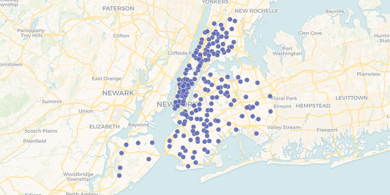
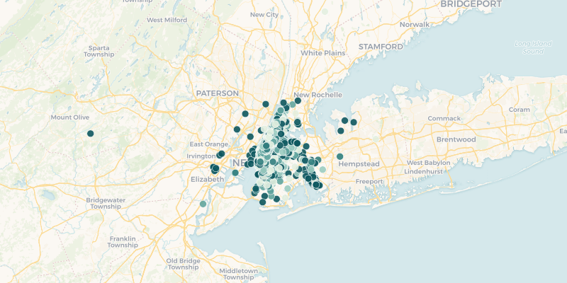
cartoframes.examples.read_mcdonalds_nyc(limit=None, **kwargs)

Read the dataset mcdonalds_nyc into a pandas DataFrame from the cartoframes example account at https://cartoframes.carto.com/tables/mcdonalds_nyc/public This dataset contains the locations of McDonald’s Fast Food within New York City.

Visually the data looks as follows:

Parameters:

• limit (int, optional) – Limit results to limit. Defaults to return all rows of the original dataset
• **kwargs – Arguments accepted in CartoContext.read

Returns:

Data in the table mcdonalds_nyc on the cartoframes example account

Return type:

pandas.DataFrame

Example:

from cartoframes.examples import read_mcdonalds_nyc
df = read_mcdonalds_nyc()

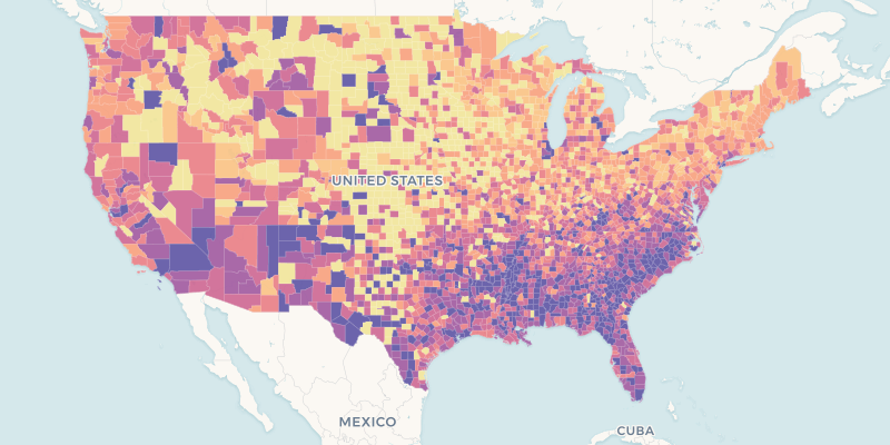
cartoframes.examples.read_nat(limit=None, **kwargs)

Read nat dataset: US county homicides 1960-1990

This table is located at: https://cartoframes.carto.com/tables/nat/public

Visually, the data looks as follows (styled by the hr90 column):

Parameters:

• limit (int, optional) – Limit results to limit. Defaults to return all rows of the original dataset
• **kwargs – Arguments accepted in CartoContext.read

Returns:

Data in the table nat on the cartoframes example account

Return type:

pandas.DataFrame

Example:

from cartoframes.examples import read_nat
df = read_nat()

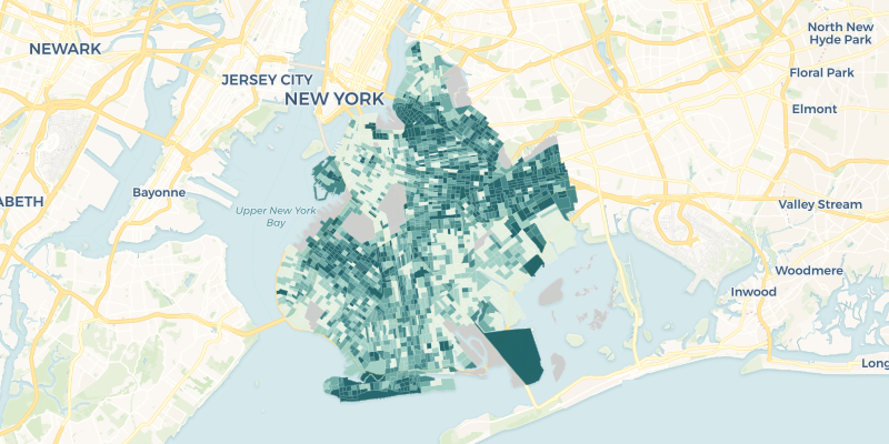
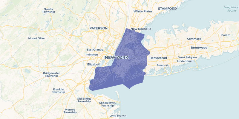
cartoframes.examples.read_nyc_census_tracts(limit=None, **kwargs)

Read the dataset nyc_census_tracts into a pandas DataFrame from the cartoframes example account at https://cartoframes.carto.com/tables/nyc_census_tracts/public This dataset contains the US census boundaries for 2015 Tiger census tracts and the corresponding GEOID in the geom_refs column.

Visually the data looks as follows:

Parameters:

• limit (int, optional) – Limit results to limit. Defaults to return all rows of the original dataset
• **kwargs – Arguments accepted in CartoContext.read

Returns:

Data in the table nyc_census_tracts on the cartoframes example account

Return type:

pandas.DataFrame

Example:

from cartoframes.examples import read_nyc_census_tracts
df = read_nyc_census_tracts()

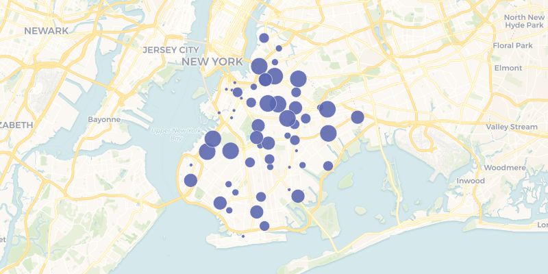
cartoframes.examples.read_taxi(limit=None, **kwargs)

Read the dataset taxi_50k into a pandas DataFrame from the cartoframes example account at https://cartoframes.carto.com/tables/taxi_50k/public. This table has a sample of 50,000 taxi trips taken in New York City. The dataset includes fare amount, tolls, payment type, and pick up and drop off locations.

Note

This dataset does not have geometries. The geometries have to be created by using the pickup or drop-off lng/lat pairs. These can be specified in CartoContext.write.

To create geometries with example_context.query, write a query such as this:

example_context.query('''
    SELECT
      CDB_LatLng(pickup_latitude, pickup_longitude) as the_geom,
      cartodb_id,
      fare_amount
    FROM
      taxi_50
''')

The data looks as follows (using the pickup location for the geometry and styling by fare_amount):

Parameters:

• limit (int, optional) – Limit results to limit. Defaults to return all rows of the original dataset
• **kwargs – Arguments accepted in CartoContext.read

Returns:

Data in the table taxi_50k on the cartoframes example account

Return type:

pandas.DataFrame

Example:

from cartoframes.examples import read_taxi
df = read_taxi()

Example CartoContext

class cartoframes.examples.Examples

A CartoContext with a CARTO account containing example data. This special CartoContext provides read access to all the datasets in the cartoframes CARTO account.

The recommended way to use this class is to import the example_context from the cartoframes.examples module:

from cartoframes.examples import example_context
df = example_context.read_taxi()

The following tables are available for use with the CartoContext.read, CartoContext.map, and CartoContext.query methods.

• brooklyn_poverty - basic poverty information for Brooklyn, New York
• mcdonalds_nyc - McDonald’s locations in New York City
• nat - historical USA-wide homicide rates at the county level
• nyc_census_tracts - Census tract boundaries for New York City
• taxi_50k - Taxi trip data, including pickup/drop-off locations. This table does not have an explicit geometry, so one must be created from the pickup_latitude/pickup_longitude columns, the dropoff_latitude/dropoff_longitude columns, or through some other process. When writing this table to your account, make sure to specify the lnglat flag in CartoContext.write

Besides the standard CartoContext methods, this class includes a convenience method for each of the tables listed above. See the full list below.

read_brooklyn_poverty(limit=None, **kwargs)

Poverty information for Brooklyn, New York, USA. See the function read_brooklyn_poverty for more information.

Example:

from cartoframes.examples import example_context
df = example_context.read_brooklyn_poverty()

read_mcdonalds_nyc(limit=None, **kwargs)

McDonald’s locations for New York City, USA. See the function read_mcdonalds_nyc for more information

Example:

from cartoframes.examples import example_context
df = example_context.read_mcdonalds_nyc()

read_nat(limit=None, **kwargs)

Historical homicide rates for the United States at the county level. See the function read_nat for more information

Example:

from cartoframes.examples import example_context
df = example_context.read_nat()

read_nyc_census_tracts(limit=None, **kwargs)

Census tracts for New York City, USA. See the function read_nyc_census_tracts for more information

Example:

from cartoframes.examples import example_context
df = example_context.read_nyc_census_tracts()

read_taxi(limit=None, **kwargs)

Taxi pickup and drop-off logs for New York City, USA. See the function read_taxi for more information

Example:

from cartoframes.examples import example_context
df = example_context.read_taxi()

contrib

contrib is an experimental library of modules in the contrib directory. These modules allow us to release new features with the expectation that they will change quickly, but give users quicker access to the bleeding edge. Most features in contrib will eventually be merged into the cartoframes core.

vector maps

This module allows users to create interactive vector maps using CARTO VL. The API for vector maps is broadly similar to CartoContext.map, with the exception that all styling expressions are expected to be straight CARTO VL expressions. See examples in the CARTO VL styling guide

Here is an example using the example CartoContext from the Examples class.

from cartoframes.examples import example_context
from cartoframes.contrib import vector
vector.vmap(
    [vector.Layer(
        'nat',
        color='ramp(globalEqIntervals($hr90, 7), sunset)',
        strokeWidth=0),
    ],
    example_context)

class cartoframes.contrib.vector.BaseMaps

Supported CARTO vector basemaps. Read more about the styles in the CARTO Basemaps repository.

darkmatter

CARTO’s “Dark Matter” style basemap

Type:str

positron

CARTO’s “Positron” style basemap

Type:str

voyager

CARTO’s “Voyager” style basemap

Type:str

Example

Create an embedded map using CARTO’s Positron style with no data layers

from cartoframes.contrib import vector
from cartoframes import CartoContext
cc = CartoContext()
vector.vmap([], context=cc, basemap=vector.BaseMaps.positron)

class cartoframes.contrib.vector.Layer(table_name, color=None, size=None, time=None, strokeColor=None, strokeWidth=None, interactivity=None)

Layer from a table name. See vector.QueryLayer for docs on the style attributes.

Example

Visualize data from a table. Here we’re using the example CartoContext. To use this with your account, replace the example_context with your CartoContext and a table in the account you authenticate against.

from cartoframes.examples import example_context
from cartoframes.contrib import vector
vector.vmap(
    [vector.Layer(
        'nat',
        color='ramp(globalEqIntervals($hr90, 7), sunset)',
        strokeWidth=0),
    ],
    example_context)

class cartoframes.contrib.vector.LocalLayer(dataframe, color=None, size=None, time=None, strokeColor=None, strokeWidth=None, interactivity=None)

Create a layer from a GeoDataFrame

TODO: add support for filepath to a GeoJSON file, JSON/dict, or string

See QueryLayer for the full styling documentation.

Example

In this example, we grab data from the cartoframes example account using read_mcdonals_nyc to get McDonald’s locations within New York City. Using the decode_geom=True argument, we decode the geometries into a form that works with GeoPandas. Finally, we pass the GeoDataFrame into LocalLayer to visualize.

import geopandas as gpd
from cartoframes.examples import read_mcdonalds_nyc, example_context
from cartoframes.contrib import vector
gdf = gpd.GeoDataFrame(read_mcdonalds_nyc(decode_geom=True))
vector.vmap([vector.LocalLayer(gdf), ], context=example_context)

class cartoframes.contrib.vector.QueryLayer(query, color=None, size=None, time=None, strokeColor=None, strokeWidth=None, interactivity=None)

CARTO VL layer based on an arbitrary query against user database

Parameters:

• query (str) – Query against user database. This query must have the following columns included to successfully have a map rendered: the_geom, the_geom_webmercator, and cartodb_id. If columns are used in styling, they must be included in this query as well.
• color (str, optional) – CARTO VL color styling for this layer. Valid inputs are simple web color names and hex values. For more advanced styling, see the CARTO VL guide on styling for more information: https://carto.com/developers/carto-vl/guides/styling-points/
• size (float or str, optional) – CARTO VL width styling for this layer if points or lines (which are not yet implemented). Valid inputs are positive numbers or text expressions involving variables. To remain consistent with cartoframes’ raster-based Layer API, size is used here in place of width, which is the CARTO VL variable name for controlling the width of a point or line. Default size is 7 pixels wide.
• time (str, optional) – Time expression to animate data. This is an alias for the CARTO VL filter style attribute. Default is no animation.
• strokeColor (str, optional) – Defines the stroke color of polygons. Default is white.
• strokeWidth (float or str, optional) – Defines the width of the stroke in pixels. Default is 1.
• interactivity (str, list, or dict, optional) –

  This option adds interactivity (click or hover) to a layer. Defaults to click if one of the following inputs are specified:

  • dict: If a dict, this must have the key cols with its value a list of columns. Optionally add event to choose hover or click. Specifying a header key/value pair adds a header to the popup that will be rendered in HTML.
  • list: A list of valid column names in the data used for this layer
  • str: A column name in the data used in this layer

Example

from cartoframes.examples import example_context
from cartoframes.contrib import vector
# create geometries from lng/lat columns
q = '''
   SELECT *, ST_Transform(the_geom, 3857) as the_geom_webmercator
   FROM (
       SELECT
         CDB_LatLng(pickup_latitude, pickup_longitude) as the_geom,
         fare_amount,
         cartodb_id
       FROM taxi_50k
   ) as _w
'''
vector.vmap(
    [vector.QueryLayer(q), ],
    example_context,
    interactivity={
        'cols': ['fare_amount', ],
        'event': 'hover'
    }
)

cartoframes.contrib.vector.vmap(*args, **kwargs)

CARTO VL-powered interactive map

Parameters:

• layers (list of Layer-types) – List of layers. One or more of Layer, QueryLayer, or LocalLayer.
• context (CartoContext) – A CartoContext instance
• basemap (str) –
  • if a str, name of a CARTO vector basemap. One of positron, voyager, or darkmatter from the BaseMaps class
  • if a dict, Mapbox or other style as the value of the style key. If a Mapbox style, the access token is the value of the token key.

Example

from cartoframes.contrib import vector
from cartoframes import CartoContext
cc = CartoContext(
    base_url='https://your_user_name.carto.com',
    api_key='your api key'
)
vector.vmap([vector.Layer('table in your account'), ], cc)

CARTO basemap style.

from cartoframes.contrib import vector
from cartoframes import CartoContext
cc = CartoContext(
    base_url='https://your_user_name.carto.com',
    api_key='your api key'
)
vector.vmap(
    [vector.Layer('table in your account'), ],
    context=cc,
    basemap=vector.BaseMaps.darkmatter
)

Custom basemap style. Here we use the Mapbox streets style, which requires an access token.

from cartoframes.contrib import vector
from cartoframes import CartoContext
cc = CartoContext(
    base_url='https://<username>.carto.com',
    api_key='your api key'
)
vector.vmap(
    [vector.Layer('table in your account'), ],
    context=cc,
    basemap={
        'style': 'mapbox://styles/mapbox/streets-v9',
        'token: '<your mapbox token>'
    }
)

Indices and tables

• Index
• Module Index
• Search Page

Version

Version:0.8.4