Cheat Sheet
For most operations below, you need to create a CartoContext object. For example, here’s how user cyclingfan with API key abc123 creates one:
from cartoframes import CartoContext
cc = CartoContext(
    base_url='https://cyclingfan.carto.com',
    api_key='abc123'
)
How to get census tracts or counties for a state
It’s a fairly common use case that someone needs the Census tracts for a region. With cartoframes you have a lot of flexibility for obtaining this data.
- Get bounding box of the region you’re interested in. Tools like Klockan’s BoundingBox tool with the CSV output are prefect. Alternatively, use a table with the appropriate covering region (e.g., an existing table with polygon(s) of Missouri, its counties, etc.).
- Get the FIPS code for the state(s) you’re interested in. The US Census provides a table as do many other sites. In this case, I’m choosing
29for Missouri.
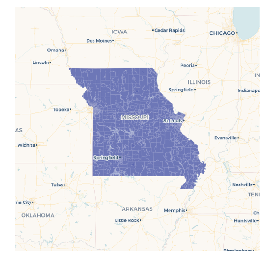
# get all census tracts (clipped by water boundaries) in specific bounding box
missouri_ct = cc.data_boundaries(
    region=[-95.774147,35.995682,-89.098846,40.613636],
    boundary='us.census.tiger.census_tract_clipped'
)

# filter out all census tracts that begin with Missouri FIPS (29)
# GEOIDs begin with two digit state FIPS, followed by three digit county FIPS
missouri_ct = missouri_ct[missouri_ct.geom_refs.str.startswith('29')]

# write to carto
cc.write(missouri_ct, 'missouri_census_tracts')

# visualize to make sure it makes sense
cc.map(Layer('missouri_census_tracts'))
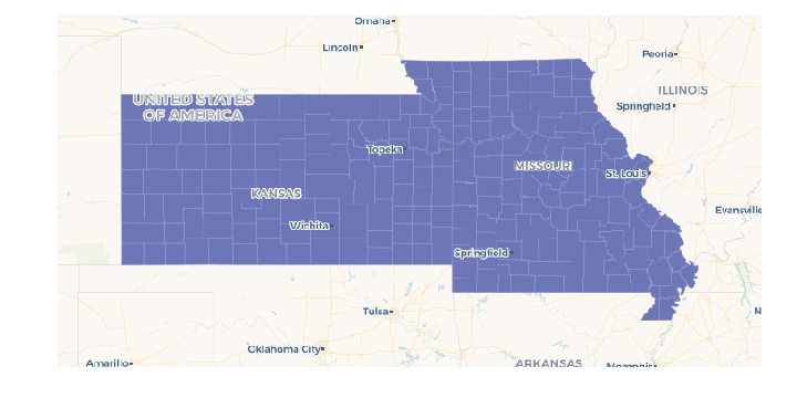
Since pandas.Series.str.startswith can take multiple string prefixes, we can filter for more than one state at a time. In this case, get all Missouri and Kansas counties:
# get all counties in bounding box around Kansas and Missouri
ks_mo_counties = cc.data_boundaries(
    region=[-102.1777729674,35.995682,-89.098846,40.613636],
    boundary='us.census.tiger.county'
)

# filter out all counties that begin with Missouri (29) or Kansas (20) FIPS
ks_mo_counties = ks_mo_counties[ks_mo_counties.geom_refs.str.startswith(('29', '20'))]

# write to carto
cc.write(ks_mo_counties, 'ks_mo_counties')

# visualize to make sure it makes sense
cc.map(Layer('ks_mo_counties'))
Get raw measures from the DO
To get raw census measures from the Data Observatory, the key part is the use of predenominated in the metadata and how=’geoid’ (or some other geom_ref) when using CartoContext.data. If you don’t use the how= flag, the Data Observatory will perform some calculations with the geometries in the table you are trying to augment.
Here we’re using a dataset with a column called geoid which has the GEOID of census tracts. Note that it’s important to specify the same geometry ID in the measure metadata as the geometries you are wishing to enrich.
- Find the measures you want, either through CartoContext.data_discovery or using the Data Observatory catalog.
- Create a dataframe with columns for each measure metadata object, or a list of dictionaries (like below) for your curated measures. Be careful to specify the specific geometry level you want the measures for and make sure the geometry reference (e.g., GEOID) you have for your geometries matches this geometry level.
# get median income for 2006 - 2010 and 2011 - 2015 five year estimates.
meta = [{
    'numer_id': 'us.census.acs.B19013001',
    'geom_id': 'us.census.tiger.census_tract',
    'normalization': 'predenominated',
    'numer_timespan': '2006 - 2010'
}, {
    'numer_id': 'us.census.acs.B19013001',
    'geom_id': 'us.census.tiger.census_tract',
    'normalization': 'predenominated',
    'numer_timespan': '2011 - 2015'
}]

boston_data = cc.data('boston_census_tracts', meta, how='geoid')
Tip
It’s best practice to keep your geometry identifiers as strings because leading zeros are removed when strings are converted to numeric types. This usually affects states with FIPS that begin with a zero, or Zip Codes in New England with leading zeros.
Engineer your DO metadata if you already have GEOID or another geom_ref
Use how=’geom_ref_col’ and specify the appropriate boundary in the metadata.
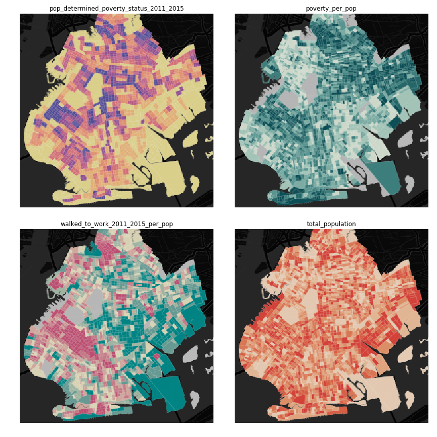
How to get a matplotlib figure with four maps
Creating a small multiple is a handy for data science visualizations for comparing data on multiple maps.
In this example, we use the example_context, so no CARTO account is required for the snippet to work.
from cartoframes import BaseMap, Layer, styling
from cartoframes.examples import example_context
import matplotlib.pyplot as plt

# table in examples account
# preview with:
#    example_context.read_brooklyn_poverty()
table = 'brooklyn_poverty'

# columns and color scheme for visualization
# view available columns with:
#    example_context.read_brooklyn_poverty().columns
cols = [('pop_determined_poverty_status_2011_2015', 'Sunset'),
        ('poverty_per_pop', 'Mint'),
        ('walked_to_work_2011_2015_per_pop', 'TealRose'),
        ('total_population', 'Peach')]

fig, axs = plt.subplots(2, 2, figsize=(8, 8))

for idx, col in enumerate(cols):
    example_context.map(layers=[BaseMap('dark'), Layer(table,
                        color={'column': col[0],
                               'scheme': styling.scheme(col[1], 7, 'quantiles')})],
          ax=axs[idx // 2][idx % 2],
          zoom=11, lng=-73.9476, lat=40.6437,
          interactive=False,
          size=(288, 288))
    axs[idx // 2][idx % 2].set_title(col[0])
fig.tight_layout()
plt.show()
Get a table as a GeoDataFrame
CARTOframes works with GeoPandas.
- For any CartoContext.read or CartoContext.query operation, use the decode_geom flag set to
True, like below. - Wrap the result of step 1 in the GeoPandas GeoDataFrame constructor
Your new GeoDataFrame will now have geometries decoded into Shapely objects that can then be used for spatial operations in your Python environment.
from cartoframes import CartoContext
import geopandas as gpd
cc = CartoContext()

gdf = gpd.GeoDataFrame(cc.read('tablename', decode_geom=True))
You can reverse this process and have geometries encoded for storage in CARTO by specifying encode_geom=True in the CartoContext.write operation.
Skip SSL verification
Some on premises installations of CARTO don’t need SSL verification. You can disable this using the requests library’s Session class and passing that into your CartoContext.
from requests import Session
session = Session()
session.verify = False

cc = CartoContext(
    base_url='https://cyclingfan.carto.com/',
    api_key='abc123',
    session=session
)
Reading large tables or queries
Sometimes tables are too large to read them out in a single CartoContext.read or CartoContext.query operation. In this case, you can read chunks and recombine, like below:
import pandas as pd

# storage for chunks of table
dfs = []

# template query
q = '''
SELECT * FROM my_big_table
WHERE cartodb_id >= {lower} and cartodb_id < {upper}
'''

num_rows = cc.sql_client.send('select count(*) from my_big_table')['rows'][0]['count']

# read in 100,000 chunks
for r in range(0, num_rows, 100000):
    dfs.append(cc.query(q.format(lower=r, upper=r+100000)))

# combine 'em all
all_together = pd.concat(dfs)
del dfs
When writing large DataFrames to CARTO, cartoframes takes care of the batching. Users shouldn’t hit errors in general until they run out of storage in their database.
Perform long running query if a time out occurs
While not a part of cartoframes yet, Batch SQL API jobs can be created through the CARTO Python SDK – the CARTO Python package for developers. Below is a sample workflow for how to perform a long running query that would otherwise produce timeout errors with CartoContext.query.
from cartoframes import CartoContext, BatchJobStatus
from carto.sql import BatchSQLClient
from time import sleep

cc = CartoContext(
    base_url='https://your-username.carto.com',
    api_key='your-api-key'
)

bsc = BatchSQLClient(cc.auth_client)

job = bsc.create(['''
    UPDATE really_big_table
    SET the_geom = cdb_geocode_street_point(direccion, ciudad, provincia, 'Spain')
    ''',
])

bjs = BatchJobStatus(cc, job)
last_status = bjs.status()['status']

while curr_status not in ('failed', 'done', 'canceled', 'unknown'):
    curr_status = bjs.status()['status']
    sleep(5)
    if curr_status != last_status:
        last_status = curr_status
        print(curr_status)

# if curr_status is 'done' the operation was successful
# and we can read the table into a dataframe
geocoded_table = cc.read('really_big_table')
Subdivide Data Observatory search region into sub-regions
Some geometries in the Data Observatory are too large, numerous, and/or complex to retrieve in one request. Census tracts (especially if they are shoreline-clipped) is one popular example. To retrieve this data, it helps to first break the search region into subregions, collect the data in each of the subregions, and then combine the data at the end. To avoid duplicate geometries along the sub-region edges, we apply the DataFrame.drop_duplicates method for the last step.
import itertools

# bbox that encompasses lower 48 states of USA
bbox = [
    -126.8220242454,
    22.991640246,
    -64.35549002,
    51.5559807141
]

# make these numbers larger if the sub-regions are not small enough
# make these numbers smaller to get more data in one call
num_divs_lng = 5
num_divs_lat = 3

delta_lng_divs = (bbox[2] - bbox[0]) / num_divs_lng
delta_lat_divs = (bbox[3] - bbox[1]) / num_divs_lat

sub_data = []
for p in itertools.product(range(num_divs_lng), range(num_divs_lat)):
    sub_bbox = (
        bbox[0] + p[0] * delta_lng_divs,
        bbox[1] + p[1] * delta_lat_divs,
        bbox[0] + (p[0] + 1) * delta_lng_divs,
        bbox[1] + (p[1] + 1) * delta_lat_divs
    )
    _df = cc.data_boundaries(
        region=sub_bbox,
        boundary='us.census.tiger.census_tract_clipped'
    )
    sub_data.append(_df)

df_all = pd.concat(sub_data)[['geom_refs', 'the_geom']]
df_all.drop_duplicates(inplace=True)
del sub_data