cartoframes.examples module

Download, preview, and query example datasets for use in cartoframes examples. Try examples by running the notebooks in binder, or trying the Example Datasets notebook.

In addition to the functions listed below, this examples module provides a CartoContext that is authenticated against all public datasets in the https://cartoframes.carto.com account. This means that besides reading the datasets from CARTO, users can also create maps from these datasets.

For example, the following will produce an interactive map of poverty rates in census tracts in Brooklyn, New York (preview of static version below code).

from cartoframes.examples import example_context
from cartoframes import Layer
example_context.map(Layer('brooklyn_poverty', color='poverty_per_pop'))

To query datasets, use the CartoContext.query method. The following example finds the poverty rate in the census tract a McDonald’s fast food joint is located (preview of static map below code).

from cartoframes.examples import import example_context

# query to get poverty rates where mcdonald's are located in brooklyn
q = '''
    SELECT m.the_geom, m.cartodb_id, m.the_geom_webmercator, c.poverty_per_pop
    FROM mcdonalds_nyc as m, brooklyn_poverty as c
    WHERE ST_Intersects(m.the_geom, c.the_geom)
'''
# get data
df = example_context.query(q)

# visualize data
from cartoframes import QueryLayer
example_context.map(QueryLayer(q, size='poverty_per_pop'))

To write datasets to your account from the examples account, the following is a good method:

from cartoframes import CartoContext
from cartoframes.examples import read_taxi
USERNAME = 'your user name'
APIKEY = 'your API key'
cc = CartoContext(
    base_url='https://{}.carto.com'.format(USERNAME),
    api_key=APIKEY
)
cc.write(
    read_taxi(),
    'taxi_data_examples_acct',
    lnglat=('pickup_latitude', 'pickup_longitude')
)

class cartoframes.examples.Examples

Bases: cartoframes.context.CartoContext

A CartoContext with a CARTO account containing example data. This special CartoContext provides read access to all the datasets in the cartoframes CARTO account.

The recommended way to use this class is to import the example_context from the cartoframes.examples module:

from cartoframes.examples import example_context
df = example_context.read_taxi()

The following tables are available for use with the CartoContext.read, CartoContext.map, and CartoContext.query methods.

• brooklyn_poverty - basic poverty information for Brooklyn, New York
• mcdonalds_nyc - McDonald’s locations in New York City
• nat - historical USA-wide homicide rates at the county level
• nyc_census_tracts - Census tract boundaries for New York City
• taxi_50k - Taxi trip data, including pickup/drop-off locations. This table does not have an explicit geometry, so one must be created from the pickup_latitude/pickup_longitude columns, the dropoff_latitude/dropoff_longitude columns, or through some other process. When writing this table to your account, make sure to specify the lnglat flag in CartoContext.write

Besides the standard CartoContext methods, this class includes a convenience method for each of the tables listed above. See the full list below.

data(table_name, metadata, persist_as=None, how='the_geom')

Get an augmented CARTO dataset with Data Observatory measures. Use CartoContext.data_discovery to search for available measures, or see the full Data Observatory catalog. Optionally persist the data as a new table.

Example

Get a DataFrame with Data Observatory measures based on the geometries in a CARTO table.

cc = cartoframes.CartoContext(BASEURL, APIKEY)
median_income = cc.data_discovery('transaction_events',
                                  regex='.*median income.*',
                                  time='2011 - 2015')
df = cc.data('transaction_events',
             median_income)

Pass in cherry-picked measures from the Data Observatory catalog. The rest of the metadata will be filled in, but it’s important to specify the geographic level as this will not show up in the column name.

median_income = [{'numer_id': 'us.census.acs.B19013001',
                  'geom_id': 'us.census.tiger.block_group',
                  'numer_timespan': '2011 - 2015'}]
df = cc.data('transaction_events', median_income)

Parameters:

• table_name (str) – Name of table on CARTO account that Data Observatory measures are to be added to.
• metadata (pandas.DataFrame) – List of all measures to add to table_name. See CartoContext.data_discovery outputs for a full list of metadata columns.
• persist_as (str, optional) – Output the results of augmenting table_name to persist_as as a persistent table on CARTO. Defaults to None, which will not create a table.
• how (str, optional) – Not fully implemented. Column name for identifying the geometry from which to fetch the data. Defaults to the_geom, which results in measures that are spatially interpolated (e.g., a neighborhood boundary’s population will be calculated from underlying census tracts). Specifying a column that has the geometry identifier (for example, GEOID for US Census boundaries), results in measures directly from the Census for that GEOID but normalized how it is specified in the metadata.

Returns:

A DataFrame representation of table_name which has new columns for each measure in metadata.

Return type:

pandas.DataFrame

Raises:

• NameError – If the columns in table_name are in the suggested_name column of metadata.
• ValueError – If metadata object is invalid or empty, or if the number of requested measures exceeds 50.
• CartoException – If user account consumes all of Data Observatory quota

data_augment(table_name, metadata)

data_boundaries(boundary=None, region=None, decode_geom=False, timespan=None, include_nonclipped=False)

Find all boundaries available for the world or a region. If boundary is specified, get all available boundary polygons for the region specified (if any). This method is espeically useful for getting boundaries for a region and, with CartoContext.data and CartoContext.data_discovery, getting tables of geometries and the corresponding raw measures. For example, if you want to analyze how median income has changed in a region (see examples section for more).

Examples

Find all boundaries available for Australia. The columns geom_name gives us the name of the boundary and geom_id is what we need for the boundary argument.

import cartoframes
cc = cartoframes.CartoContext('base url', 'api key')
au_boundaries = cc.data_boundaries(region='Australia')
au_boundaries[['geom_name', 'geom_id']]

Get the boundaries for Australian Postal Areas and map them.

from cartoframes import Layer
au_postal_areas = cc.data_boundaries(boundary='au.geo.POA')
cc.write(au_postal_areas, 'au_postal_areas')
cc.map(Layer('au_postal_areas'))

Get census tracts around Idaho Falls, Idaho, USA, and add median income from the US census. Without limiting the metadata, we get median income measures for each census in the Data Observatory.

cc = cartoframes.CartoContext('base url', 'api key')
# will return DataFrame with columns `the_geom` and `geom_ref`
tracts = cc.data_boundaries(
    boundary='us.census.tiger.census_tract',
    region=[-112.096642,43.429932,-111.974213,43.553539])
# write geometries to a CARTO table
cc.write(tracts, 'idaho_falls_tracts')
# gather metadata needed to look up median income
median_income_meta = cc.data_discovery(
    'idaho_falls_tracts',
    keywords='median income',
    boundaries='us.census.tiger.census_tract')
# get median income data and original table as new dataframe
idaho_falls_income = cc.data(
    'idaho_falls_tracts',
    median_income_meta,
    how='geom_refs')
# overwrite existing table with newly-enriched dataframe
cc.write(idaho_falls_income,
         'idaho_falls_tracts',
         overwrite=True)

Parameters:

• boundary (str, optional) – Boundary identifier for the boundaries that are of interest. For example, US census tracts have a boundary ID of us.census.tiger.census_tract, and Brazilian Municipios have an ID of br.geo.municipios. Find IDs by running CartoContext.data_boundaries without any arguments, or by looking in the Data Observatory catalog.
• region (str, optional) –

  Region where boundary information or, if boundary is specified, boundary polygons are of interest. region can be one of the following:

  • table name (str): Name of a table in user’s CARTO account
  • bounding box (list of float): List of four values (two lng/lat pairs) in the following order: western longitude, southern latitude, eastern longitude, and northern latitude. For example, Switzerland fits in [5.9559111595,45.8179931641,10.4920501709,47.808380127]

• timespan (str, optional) – Specific timespan to get geometries from. Defaults to use the most recent. See the Data Observatory catalog for more information.
• decode_geom (bool, optional) – Whether to return the geometries as Shapely objects or keep them encoded as EWKB strings. Defaults to False.
• include_nonclipped (bool, optional) – Optionally include non-shoreline-clipped boundaries. These boundaries are the raw boundaries provided by, for example, US Census Tiger.

Returns:

If boundary is specified, then all available boundaries and accompanying geom_refs in region (or the world if region is None or not specified) are returned. If boundary is not specified, then a DataFrame of all available boundaries in region (or the world if region is None)

Return type:

pandas.DataFrame

data_discovery(region, keywords=None, regex=None, time=None, boundaries=None, include_quantiles=False)

Discover Data Observatory measures. This method returns the full Data Observatory metadata model for each measure or measures that match the conditions from the inputs. The full metadata in each row uniquely defines a measure based on the timespan, geographic resolution, and normalization (if any). Read more about the metadata response in Data Observatory documentation.

Internally, this method finds all measures in region that match the conditions set in keywords, regex, time, and boundaries (if any of them are specified). Then, if boundaries is not specified, a geographical resolution for that measure will be chosen subject to the type of region specified:

1. If region is a table name, then a geographical resolution that is roughly equal to region size / number of subunits.
2. If region is a country name or bounding box, then a geographical resolution will be chosen roughly equal to region size / 500.

Since different measures are in some geographic resolutions and not others, different geographical resolutions for different measures are oftentimes returned.

Tip

To remove the guesswork in how geographical resolutions are selected, specify one or more boundaries in boundaries. See the boundaries section for each region in the Data Observatory catalog.

The metadata returned from this method can then be used to create raw tables or for augmenting an existing table from these measures using CartoContext.data. For the full Data Observatory catalog, visit https://cartodb.github.io/bigmetadata/. When working with the metadata DataFrame returned from this method, be careful to only remove rows not columns as CartoContext.data <cartoframes.context.CartoContext.data> generally needs the full metadata.

Note

Narrowing down a discovery query using the keywords, regex, and time filters is important for getting a manageable metadata set. Besides there being a large number of measures in the DO, a metadata response has acceptable combinations of measures with demonimators (normalization and density), and the same measure from other years.

For example, setting the region to be United States counties with no filter values set will result in many thousands of measures.

Examples

Get all European Union measures that mention freight.

meta = cc.data_discovery('European Union',
                         keywords='freight',
                         time='2010')
print(meta['numer_name'].values)

Parameters:

• region (str or list of float) –

  Information about the region of interest. region can be one of three types:

  • region name (str): Name of region of interest. Acceptable values are limited to: ‘Australia’, ‘Brazil’, ‘Canada’, ‘European Union’, ‘France’, ‘Mexico’, ‘Spain’, ‘United Kingdom’, ‘United States’.
  • table name (str): Name of a table in user’s CARTO account with geometries. The region will be the bounding box of the table.

    Note

    If a table name is also a valid Data Observatory region name, the Data Observatory name will be chosen over the table.

  • bounding box (list of float): List of four values (two lng/lat pairs) in the following order: western longitude, southern latitude, eastern longitude, and northern latitude. For example, Switzerland fits in [5.9559111595,45.8179931641,10.4920501709,47.808380127]

  Note

  Geometry levels are generally chosen by subdividing the region into the next smallest administrative unit. To override this behavior, specify the boundaries flag. For example, set boundaries to 'us.census.tiger.census_tract' to choose US census tracts.

• keywords (str or list of str, optional) – Keyword or list of keywords in measure description or name. Response will be matched on all keywords listed (boolean or).
• regex (str, optional) – A regular expression to search the measure descriptions and names. Note that this relies on PostgreSQL’s case insensitive operator ~*. See PostgreSQL docs for more information.
• boundaries (str or list of str, optional) – Boundary or list of boundaries that specify the measure resolution. See the boundaries section for each region in the Data Observatory catalog.
• include_quantiles (bool, optional) – Include quantiles calculations which are a calculation of how a measure compares to all measures in the full dataset. Defaults to False. If True, quantiles columns will be returned for each column which has it pre-calculated.

Returns:

A dataframe of the complete metadata model for specific measures based on the search parameters.

Return type:

pandas.DataFrame

Raises:

• ValueError – If region is a list and does not consist of four elements, or if region is not an acceptable region
• CartoException – If region is not a table in user account

read_brooklyn_poverty(limit=None, **kwargs)

Poverty information for Brooklyn, New York, USA. See the function read_brooklyn_poverty for more information.

Example:

from cartoframes.examples import example_context
df = example_context.read_brooklyn_poverty()

read_mcdonalds_nyc(limit=None, **kwargs)

McDonald’s locations for New York City, USA. See the function read_mcdonalds_nyc for more information

Example:

from cartoframes.examples import example_context
df = example_context.read_mcdonalds_nyc()

read_nat(limit=None, **kwargs)

Historical homicide rates for the United States at the county level. See the function read_nat for more information

Example:

from cartoframes.examples import example_context
df = example_context.read_nat()

read_ne_50m_graticules_15(limit=None, **kwargs)

50m world Mercator grid <cartoframes.examples.read_ne_50m_graticules_15>` for more information.

Example:

from cartoframes.examples import example_context
df = example_context.read_ne_50m_graticules_15()

read_nyc_census_tracts(limit=None, **kwargs)

Census tracts for New York City, USA. See the function read_nyc_census_tracts for more information

Example:

from cartoframes.examples import example_context
df = example_context.read_nyc_census_tracts()

read_taxi(limit=None, **kwargs)

Taxi pickup and drop-off logs for New York City, USA. See the function read_taxi for more information

Example:

from cartoframes.examples import example_context
df = example_context.read_taxi()

write(df, table_name, temp_dir=None, overwrite=False, lnglat=None, encode_geom=False, geom_col=None, **kwargs)

Write a DataFrame to a CARTO table.

Examples

Write a pandas DataFrame to CARTO.

cc.write(df, 'brooklyn_poverty', overwrite=True)

Scrape an HTML table from Wikipedia and send to CARTO with content guessing to create a geometry from the country column. This uses a CARTO Import API param content_guessing parameter.

url = 'https://en.wikipedia.org/wiki/List_of_countries_by_life_expectancy'
# retrieve first HTML table from that page
df = pd.read_html(url, header=0)[0]
# send to carto, let it guess polygons based on the 'country'
#   column. Also set privacy to 'public'
cc.write(df, 'life_expectancy',
         content_guessing=True,
         privacy='public')
cc.map(layers=Layer('life_expectancy',
                    color='both_sexes_life_expectancy'))

Warning

datetime64[ns] column will lose precision sending a dataframe to CARTO because postgresql has millisecond resolution while pandas does nanoseconds

Parameters:

• df (pandas.DataFrame) – DataFrame to write to table_name in user CARTO account
• table_name (str) – Table to write df to in CARTO.
• temp_dir (str, optional) – Directory for temporary storage of data that is sent to CARTO. Defaults are defined by appdirs.
• overwrite (bool, optional) – Behavior for overwriting table_name if it exits on CARTO. Defaults to False.
• lnglat (tuple, optional) – lng/lat pair that can be used for creating a geometry on CARTO. Defaults to None. In some cases, geometry will be created without specifying this. See CARTO’s Import API for more information.
• encode_geom (bool, optional) – Whether to write geom_col to CARTO as the_geom.
• geom_col (str, optional) – The name of the column where geometry information is stored. Used in conjunction with encode_geom.
• **kwargs –

  Keyword arguments to control write operations. Options are:

  • compression to set compression for files sent to CARTO. This will cause write speedups depending on the dataset. Options are None (no compression, default) or gzip.
  • Some arguments from CARTO’s Import API. See the params listed in the documentation for more information. For example, when using content_guessing=’true’, a column named ‘countries’ with country names will be used to generate polygons for each country. Another use is setting the privacy of a dataset. To avoid unintended consequences, avoid file, url, and other similar arguments.

Returns:

Dataset

Note

DataFrame indexes are changed to ordinary columns. CARTO creates an index called cartodb_id for every table that runs from 1 to the length of the DataFrame.

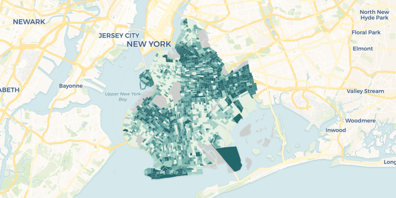
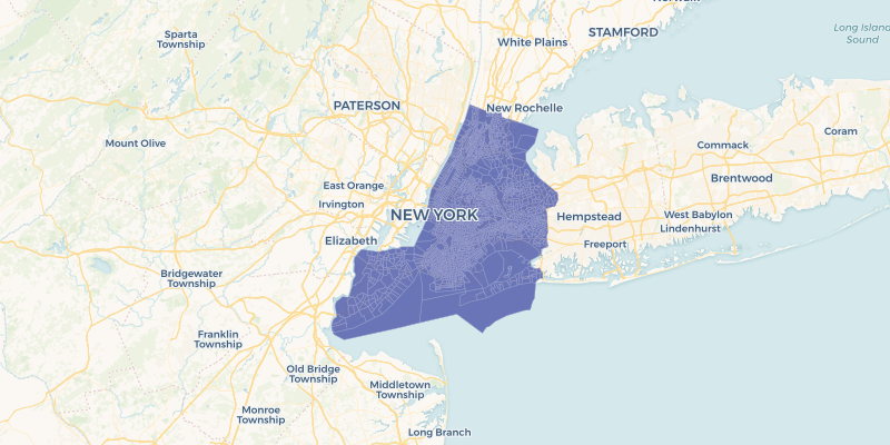
cartoframes.examples.read_brooklyn_poverty(limit=None, **kwargs)

Read the dataset brooklyn_poverty into a pandas DataFrame from the cartoframes example account at https://cartoframes.carto.com/tables/brooklyn_poverty/public This dataset contains poverty rates for census tracts in Brooklyn, New York

The data looks as follows (styled on poverty_per_pop):

Parameters:

• limit (int, optional) – Limit results to limit. Defaults to return all rows of the original dataset
• **kwargs – Arguments accepted in CartoContext.read

Returns:

Data in the table brooklyn_poverty on the cartoframes example account

Return type:

pandas.DataFrame

Example:

from cartoframes.examples import read_brooklyn_poverty
df = read_brooklyn_poverty()

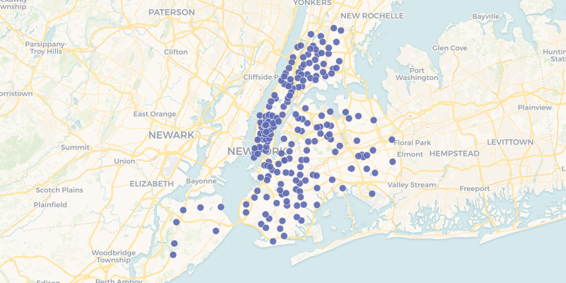
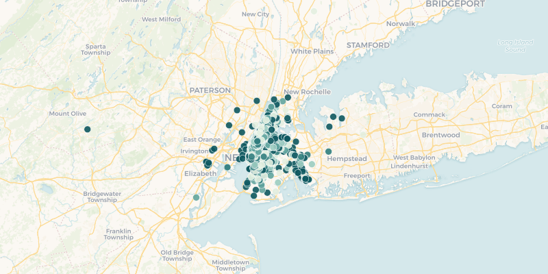
cartoframes.examples.read_mcdonalds_nyc(limit=None, **kwargs)

Read the dataset mcdonalds_nyc into a pandas DataFrame from the cartoframes example account at https://cartoframes.carto.com/tables/mcdonalds_nyc/public This dataset contains the locations of McDonald’s Fast Food within New York City.

Visually the data looks as follows:

Parameters:

• limit (int, optional) – Limit results to limit. Defaults to return all rows of the original dataset
• **kwargs – Arguments accepted in CartoContext.read

Returns:

Data in the table mcdonalds_nyc on the cartoframes example account

Return type:

pandas.DataFrame

Example:

from cartoframes.examples import read_mcdonalds_nyc
df = read_mcdonalds_nyc()

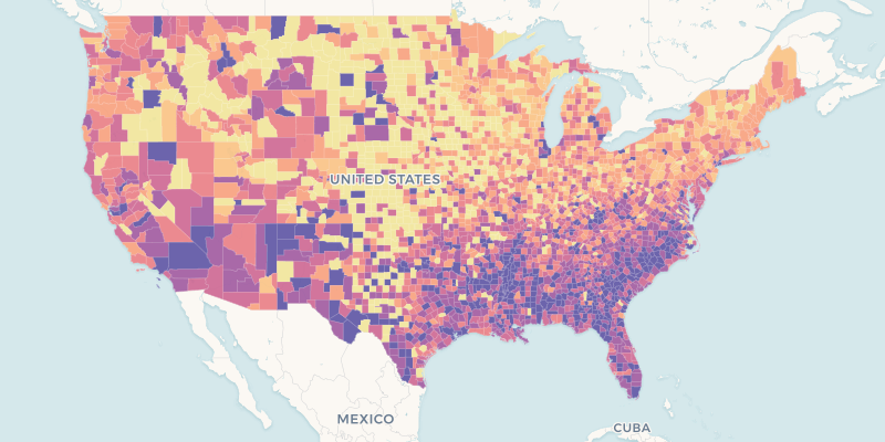
cartoframes.examples.read_nat(limit=None, **kwargs)

Read nat dataset: US county homicides 1960-1990

This table is located at: https://cartoframes.carto.com/tables/nat/public

Visually, the data looks as follows (styled by the hr90 column):

Parameters:

• limit (int, optional) – Limit results to limit. Defaults to return all rows of the original dataset
• **kwargs – Arguments accepted in CartoContext.read

Returns:

Data in the table nat on the cartoframes example account

Return type:

pandas.DataFrame

Example:

from cartoframes.examples import read_nat
df = read_nat()

cartoframes.examples.read_ne_50m_graticules_15(limit=None, **kwargs)

Read the dataset ne_50m_graticules_15 into a pandas DataFrame from the cartoframes example account at https://cartoframes.carto.com/tables/ne_50m_graticules_15/public This dataset contains a 50m world Mercator grid

Parameters:

• limit (int, optional) – Limit results to limit. Defaults to return all rows of the original dataset
• **kwargs – Arguments accepted in CartoContext.read

Returns:

Data in the table ne_50m_graticules_15 on the cartoframes example account

Return type:

pandas.DataFrame

Example:

from cartoframes.examples import read_ne_50m_graticules_15
df = read_ne_50m_graticules_15()

cartoframes.examples.read_nyc_census_tracts(limit=None, **kwargs)

Read the dataset nyc_census_tracts into a pandas DataFrame from the cartoframes example account at https://cartoframes.carto.com/tables/nyc_census_tracts/public This dataset contains the US census boundaries for 2015 Tiger census tracts and the corresponding GEOID in the geom_refs column.

Visually the data looks as follows:

Parameters:

• limit (int, optional) – Limit results to limit. Defaults to return all rows of the original dataset
• **kwargs – Arguments accepted in CartoContext.read

Returns:

Data in the table nyc_census_tracts on the cartoframes example account

Return type:

pandas.DataFrame

Example:

from cartoframes.examples import read_nyc_census_tracts
df = read_nyc_census_tracts()

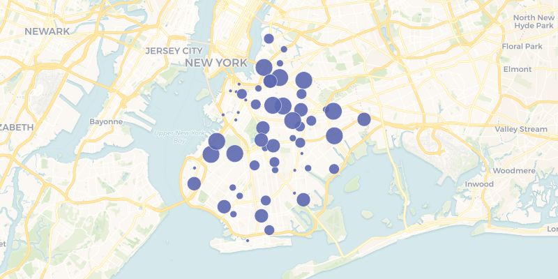
cartoframes.examples.read_taxi(limit=None, **kwargs)

Read the dataset taxi_50k into a pandas DataFrame from the cartoframes example account at https://cartoframes.carto.com/tables/taxi_50k/public. This table has a sample of 50,000 taxi trips taken in New York City. The dataset includes fare amount, tolls, payment type, and pick up and drop off locations.

Note

This dataset does not have geometries. The geometries have to be created by using the pickup or drop-off lng/lat pairs. These can be specified in CartoContext.write.

To create geometries with example_context.query, write a query such as this:

example_context.query('''
    SELECT
      CDB_LatLng(pickup_latitude, pickup_longitude) as the_geom,
      cartodb_id,
      fare_amount
    FROM
      taxi_50
''')

The data looks as follows (using the pickup location for the geometry and styling by fare_amount):

Parameters:

• limit (int, optional) – Limit results to limit. Defaults to return all rows of the original dataset
• **kwargs – Arguments accepted in CartoContext.read

Returns:

Data in the table taxi_50k on the cartoframes example account

Return type:

pandas.DataFrame

Example:

from cartoframes.examples import read_taxi
df = read_taxi()